US Elections

Biden’s Approval Margins
This assignment involves analyzing the poll approval for the US president. Here, I’ll again start by loading the libraries which I might need to do my analysis: and a bit of cleaning the data:
# Imported approval polls data directly off fivethirtyeight website
approval_polllist <- read_csv('https://projects.fivethirtyeight.com/biden-approval-data/approval_polllist.csv')
##
## ── Column specification ────────────────────────────────────────────────────────
## cols(
## .default = col_character(),
## samplesize = col_double(),
## weight = col_double(),
## influence = col_double(),
## approve = col_double(),
## disapprove = col_double(),
## adjusted_approve = col_double(),
## adjusted_disapprove = col_double(),
## tracking = col_logical(),
## poll_id = col_double(),
## question_id = col_double()
## )
## ℹ Use `spec()` for the full column specifications.glimpse(approval_polllist)## Rows: 1,598
## Columns: 22
## $ president <chr> "Joseph R. Biden Jr.", "Joseph R. Biden Jr.", "Jos…
## $ subgroup <chr> "All polls", "All polls", "All polls", "All polls"…
## $ modeldate <chr> "9/13/2021", "9/13/2021", "9/13/2021", "9/13/2021"…
## $ startdate <chr> "1/21/2021", "1/26/2021", "1/26/2021", "1/27/2021"…
## $ enddate <chr> "2/2/2021", "1/28/2021", "1/28/2021", "1/29/2021",…
## $ pollster <chr> "Gallup", "Morning Consult", "Rasmussen Reports/Pu…
## $ grade <chr> "B+", "B", "B", "A+", "B", "B", "B+", "B-", "B/C",…
## $ samplesize <dbl> 906.00, 3423.00, 1500.00, 1261.00, 2200.00, 15000.…
## $ population <chr> "a", "a", "lv", "a", "a", "a", "rv", "rv", "lv", "…
## $ weight <dbl> 1.31470660, 0.19383147, 0.33818752, 2.35547250, 0.…
## $ influence <dbl> 0, 0, 0, 0, 0, 0, 0, 0, 0, 0, 0, 0, 0, 0, 0, 0, 0,…
## $ approve <dbl> 57.00000, 56.00000, 50.00000, 53.00000, 56.00000, …
## $ disapprove <dbl> 37.0, 31.0, 45.0, 29.0, 33.0, 32.0, 39.0, 35.0, 36…
## $ adjusted_approve <dbl> 56.36684, 54.58655, 52.41459, 53.38782, 54.58655, …
## $ adjusted_disapprove <dbl> 36.35828, 34.25346, 39.04388, 33.12161, 36.25346, …
## $ multiversions <chr> NA, NA, NA, NA, NA, NA, NA, NA, NA, NA, "*", NA, N…
## $ tracking <lgl> NA, NA, TRUE, NA, NA, TRUE, NA, NA, NA, TRUE, TRUE…
## $ url <chr> "https://news.gallup.com/poll/329348/biden-begins-…
## $ poll_id <dbl> 74344, 74292, 74290, 74321, 74378, 74339, 74322, 7…
## $ question_id <dbl> 139651, 139518, 139515, 139560, 139765, 139644, 13…
## $ createddate <chr> "2/4/2021", "2/1/2021", "1/29/2021", "2/1/2021", "…
## $ timestamp <chr> "13:37:08 13 Sep 2021", "13:37:08 13 Sep 2021", "1…#Using `lubridate` to fix dates, as they are given as characters.
approval_polllist <- approval_polllist %>%
mutate(enddate = mdy(enddate))What I did is to calculate the average net approval rate (approve- disapprove) for each week since he got into office. I plot the net approval, along with its 95% confidence interval. There are various dates given for each poll, I used enddate, i.e., the date the poll ended.
#tidy data and calculate CI using formula
net_approval <- approval_polllist %>%
  filter(!is.na(subgroup)) %>%
  #using lubridate to get week number
  mutate(week = isoweek(enddate),
         net_approval_day = approve - disapprove) %>%
  group_by(subgroup, week) %>%
  summarise(mean_net_approval = mean(net_approval_day),
            sd_net_approval = sd(net_approval_day),
            count = n(),
            se_twitter = sd_net_approval / sqrt(count),
            t_critical = qt(0.975, count - 1),
            lower_ci =  mean_net_approval - t_critical*se_twitter,
            upper_ci = mean_net_approval + t_critical*se_twitter)
## Warning in qt(0.975, count - 1): NaNs produced
## Warning in qt(0.975, count - 1): NaNs produced## `summarise()` has grouped output by 'subgroup'. You can override using the `.groups` argument.#plot Biden's weekly net approval rate
ggplot(net_approval,
aes(x= week,
y= mean_net_approval)) +
geom_line(color = "red")+
geom_point(color = "red")+
geom_smooth(color = "blue",
level = 0,
size = 1)+
#add orange line at zero
geom_hline(yintercept=0,
color = "orange",
size = 2)+
theme_bw()+
#add confidence band using calculated CI
geom_ribbon(aes(ymin = lower_ci,
ymax = upper_ci),
alpha=0.3,
fill = "grey",
color = "red") +
labs(
title = "Estimating Approval Margin (approve-disapprove) for Joe Biden",
subtitle = "Weekly average of all polls by different subgroups",
x = "Week of the year",
y = "Average Approval Margin (approve-disapprove)")+
#differentiate between Adults, All polls, Voters
facet_wrap(vars(subgroup))+
scale_y_continuous(breaks=seq(-15,10,2.5))## `geom_smooth()` using method = 'loess' and formula 'y ~ x'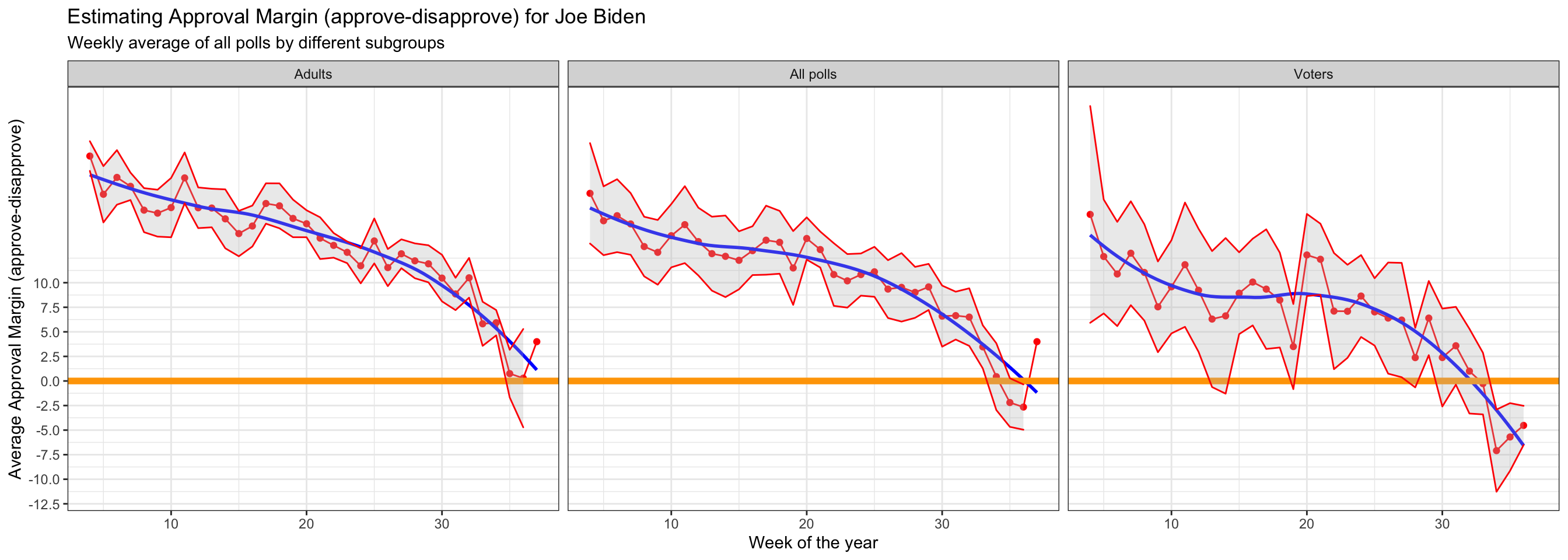
Compare Confidence Intervals
Compare the confidence intervals for week 4 and week 25.
net_approval_4_25 <- net_approval %>%
  filter(week %in% c(4, 25)) %>%
  mutate(
    ci_width = upper_ci - lower_ci) %>%
  select(subgroup, week, lower_ci, upper_ci, ci_width)

net_approval_4_25
## # A tibble: 6 x 5
## # Groups: subgroup [3]
## subgroup week lower_ci upper_ci ci_width
## <chr> <dbl> <dbl> <dbl> <dbl>
## 1 Adults 4 21.4 24.4 3.02
## 2 Adults 25 12.0 16.5 4.57
## 3 All polls 4 14.0 24.2 10.2
## 4 All polls 25 8.57 13.7 5.08
## 5 Voters 4 5.92 28.0 22.1
## 6 Voters 25 3.61 10.5 6.85From the results, I can clearly see that for all subgroups, the confidence interval for Biden’s net approval rate has been narrower from week 4 to week 25. Especially for Voters subgroup, the width confidence interval has been drastically decreased from 16.84 to 6.85. I assume this is because as after Biden has been elected for a longer period of time in week 25 (almost half a year), all adults including his voters would become more clear about their approval or disapproval to the president. After Americans took over 25-week time to evaluate their new elected president, they would probably have a clearer attitude towards Biden’s policy changes, administration and national strategies. These clearer perceptions then result in this decreasing confidence interval trend.