
Like always, I’ll start this project too with loading the required libraries:
url <- "https://happiness-report.s3.amazonaws.com/2021/DataPanelWHR2021C2.xls"
# Download data to temporary file
httr::GET(url, write_disk(happiness.temp <- tempfile(fileext = ".xls")))
## Response [https://happiness-report.s3.amazonaws.com/2021/DataPanelWHR2021C2.xls]
##   Date: 2021-09-20 19:48
##   Status: 200
##   Content-Type: application/vnd.ms-excel
##   Size: 435 kB
## <ON DISK>  /var/folders/1k/wft4clgd33qdzxt_l3hlsfqh0000gn/T//Rtmp9OoYov/file276d52deb01f.xls
Before starting with our statistocs and regression models, lets just have a look at our data:
# Using read_excel to read it as dataframe
world_happiness <- read_excel(happiness.temp,
                    sheet = "Sheet1",
                    range = cell_cols("A:K")) %>%
  janitor::clean_names()

# inspect dataframe
glimpse(world_happiness)
## Rows: 1,949
## Columns: 11
## $ country_name                     <chr> "Afghanistan", "Afghanistan", "Afghan…
## $ year                             <dbl> 2008, 2009, 2010, 2011, 2012, 2013, 2…
## $ life_ladder                      <dbl> 3.723590, 4.401778, 4.758381, 3.83171…
## $ log_gdp_per_capita               <dbl> 7.370100, 7.539972, 7.646709, 7.61953…
## $ social_support                   <dbl> 0.4506623, 0.5523084, 0.5390752, 0.52…
## $ healthy_life_expectancy_at_birth <dbl> 50.80, 51.20, 51.60, 51.92, 52.24, 52…
## $ freedom_to_make_life_choices     <dbl> 0.7181143, 0.6788964, 0.6001272, 0.49…
## $ generosity                       <dbl> 0.167639986, 0.190099195, 0.120589636…
## $ perceptions_of_corruption        <dbl> 0.8816863, 0.8500354, 0.7067661, 0.73…
## $ positive_affect                  <dbl> 0.5176372, 0.5839256, 0.6182655, 0.61…
## $ negative_affect                  <dbl> 0.2581955, 0.2370924, 0.2753238, 0.26…
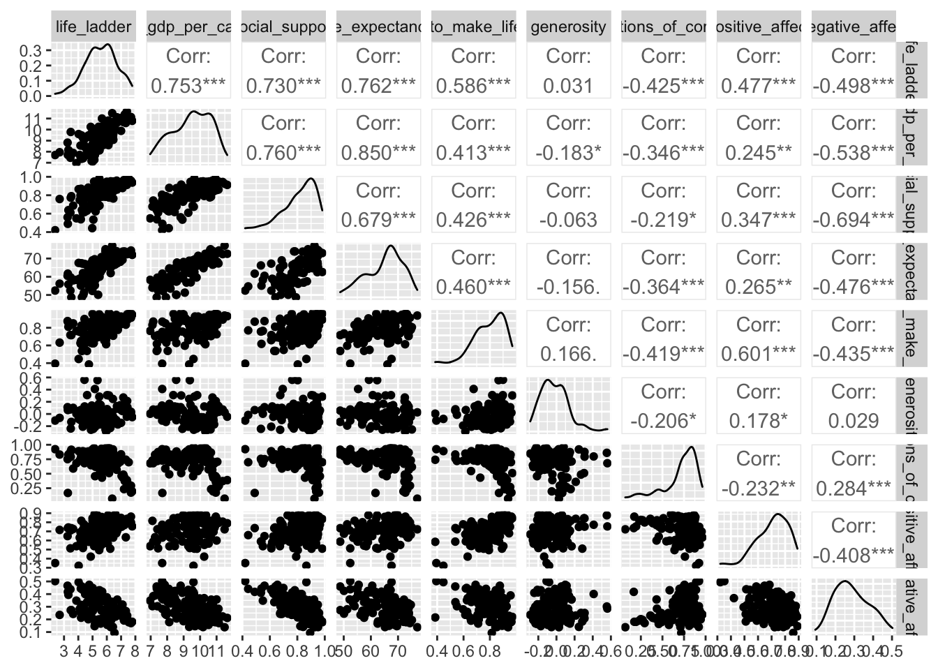
I have used ggparis to analyze the correlation between dependent and explanatory variables:
# Scatterplot-correlation matrix for 2019 using GGally::ggpairs()
world_happiness_19 <- world_happiness %>%
  filter(year==2019)

world_happiness_19 %>%
  select(-c(country_name,year)) %>%
  ggpairs(alpha = 0.3)
# Summary statistics for life_ladder, a measure of happiness score
world_happiness_19 %>%
  select(life_ladder) %>%
  skim()
Table 1: Data summary
| Name |
Piped data |
| Number of rows |
144 |
| Number of columns |
1 |
| _______________________ |
|
| Column type frequency: |
|
| numeric |
1 |
| ________________________ |
|
| Group variables |
None |
Variable type: numeric
| life_ladder |
0 |
1 |
5.57 |
1.11 |
2.38 |
4.93 |
5.59 |
6.28 |
7.78 |
▁▃▇▇▃ |
Regression Models
# fit 3 models, with model1 being just the average happiness
model1 <- lm(life_ladder ~ 1, data = world_happiness_19)
mosaic::msummary(model1)
## Registered S3 method overwritten by 'mosaic':
##   method                           from
##   fortify.SpatialPolygonsDataFrame ggplot2
##             Estimate Std. Error t value Pr(>|t|)
## (Intercept)  5.57089    0.09266   60.12   <2e-16 ***
##
## Residual standard error: 1.112 on 143 degrees of freedom
model2 <- lm(life_ladder ~ freedom_to_make_life_choices, data = world_happiness_19)
mosaic::msummary(model2)
##                              Estimate Std. Error t value Pr(>|t|)
## (Intercept)                    1.1235     0.5233   2.147   0.0335 *
## freedom_to_make_life_choices   5.5982     0.6516   8.591 1.46e-14 ***
##
## Residual standard error: 0.9072 on 141 degrees of freedom
##   (1 observation deleted due to missingness)
## Multiple R-squared:  0.3436, Adjusted R-squared:  0.3389
## F-statistic: 73.81 on 1 and 141 DF,  p-value: 1.456e-14
model3 <- lm(life_ladder ~ log_gdp_per_capita + freedom_to_make_life_choices, data = world_happiness_19)
mosaic::msummary(model3)
##                              Estimate Std. Error t value Pr(>|t|)
## (Intercept)                  -2.71600    0.52309  -5.192 7.53e-07 ***
## log_gdp_per_capita            0.61363    0.05478  11.201  < 2e-16 ***
## freedom_to_make_life_choices  3.11083    0.53828   5.779 5.01e-08 ***
##
## Residual standard error: 0.6643 on 134 degrees of freedom
##   (7 observations deleted due to missingness)
## Multiple R-squared:  0.6565, Adjusted R-squared:  0.6513
## F-statistic:   128 on 2 and 134 DF,  p-value: < 2.2e-16
model4 <- lm(life_ladder ~ log_gdp_per_capita + social_support + freedom_to_make_life_choices, data = world_happiness_19)
mosaic::msummary(model4)
##                              Estimate Std. Error t value Pr(>|t|)
## (Intercept)                   -2.6830     0.4939  -5.432 2.57e-07 ***
## log_gdp_per_capita             0.3909     0.0744   5.254 5.76e-07 ***
## social_support                 2.9973     0.7198   4.164 5.59e-05 ***
## freedom_to_make_life_choices   2.6539     0.5199   5.105 1.12e-06 ***
##
## Residual standard error: 0.6272 on 133 degrees of freedom
##   (7 observations deleted due to missingness)
## Multiple R-squared:  0.6961, Adjusted R-squared:  0.6892
## F-statistic: 101.5 on 3 and 133 DF,  p-value: < 2.2e-16
model5 <- lm(life_ladder ~ log_gdp_per_capita + healthy_life_expectancy_at_birth + social_support + freedom_to_make_life_choices, data = world_happiness_19)
mosaic::msummary(model5)
##                                  Estimate Std. Error t value Pr(>|t|)
## (Intercept)                      -3.41409    0.52970  -6.445 2.06e-09 ***
## log_gdp_per_capita                0.18468    0.10084   1.831 0.069337 .
## healthy_life_expectancy_at_birth  0.04847    0.01543   3.142 0.002079 **
## social_support                    2.80793    0.70049   4.009 0.000102 ***
## freedom_to_make_life_choices      2.26060    0.51739   4.369 2.53e-05 ***
##
## Residual standard error: 0.6075 on 130 degrees of freedom
##   (9 observations deleted due to missingness)
## Multiple R-squared:  0.7202, Adjusted R-squared:  0.7116
## F-statistic: 83.65 on 4 and 130 DF,  p-value: < 2.2e-16
# if we want regression summary in tibble format, use broom::tidy() and broom::glance()
# get model summary and R2, etc for both models
model2 %>% broom::tidy(conf.int = TRUE)
| term | estimate | std.error | statistic | p.value | conf.low | conf.high |
| (Intercept) | 1.12 | 0.523 | 2.15 | 0.0335 | 0.089 | 2.16 |
| freedom_to_make_life_choices | 5.6 | 0.652 | 8.59 | 1.46e-14 | 4.31 | 6.89 |
model2 %>% broom::glance()
| r.squared | adj.r.squared | sigma | statistic | p.value | df | logLik | AIC | BIC | deviance | df.residual | nobs |
| 0.344 | 0.339 | 0.907 | 73.8 | 1.46e-14 | 1 | -188 | 382 | 391 | 116 | 141 | 143 |
model3 %>% broom::tidy(conf.int = TRUE)
| term | estimate | std.error | statistic | p.value | conf.low | conf.high |
| (Intercept) | -2.72 | 0.523 | -5.19 | 7.53e-07 | -3.75 | -1.68 |
| log_gdp_per_capita | 0.614 | 0.0548 | 11.2 | 5.81e-21 | 0.505 | 0.722 |
| freedom_to_make_life_choices | 3.11 | 0.538 | 5.78 | 5.01e-08 | 2.05 | 4.18 |
model3 %>% broom::glance()
| r.squared | adj.r.squared | sigma | statistic | p.value | df | logLik | AIC | BIC | deviance | df.residual | nobs |
| 0.656 | 0.651 | 0.664 | 128 | 8.15e-32 | 2 | -137 | 282 | 293 | 59.1 | 134 | 137 |
# produce summary table comparing models using huxtable::huxreg()
huxreg(model1, model2, model3, model4,model5,
       statistics = c('#observations' = 'nobs',
                      'R squared' = 'r.squared',
                      'Adj. R Squared' = 'adj.r.squared',
                      'Residual SE' = 'sigma'),
       bold_signif = 0.05,
       stars = NULL
) %>%
  set_caption('Comparison of models')
Comparison of models
| (1) | (2) | (3) | (4) | (5) |
| (Intercept) | 5.571 | 1.123 | -2.716 | -2.683 | -3.414 |
| (0.093) | (0.523) | (0.523) | (0.494) | (0.530) |
| freedom_to_make_life_choices | | 5.598 | 3.111 | 2.654 | 2.261 |
| | (0.652) | (0.538) | (0.520) | (0.517) |
| log_gdp_per_capita | | | 0.614 | 0.391 | 0.185 |
| | | (0.055) | (0.074) | (0.101) |
| social_support | | | | 2.997 | 2.808 |
| | | | (0.720) | (0.700) |
| healthy_life_expectancy_at_birth | | | | | 0.048 |
| | | | | (0.015) |
| #observations | 144 | 143 | 137 | 137 | 135 |
| R squared | 0.000 | 0.344 | 0.656 | 0.696 | 0.720 |
| Adj. R Squared | 0.000 | 0.339 | 0.651 | 0.689 | 0.712 |
| Residual SE | 1.112 | 0.907 | 0.664 | 0.627 | 0.607 |
# Check whether any model has a VIF (Variance Inflation Factor) greater than 5
car::vif(model3)
##           log_gdp_per_capita freedom_to_make_life_choices
##                     1.205776                     1.205776
car::vif(model4)
##           log_gdp_per_capita               social_support
##                     2.495287                     2.568193
## freedom_to_make_life_choices
##                     1.261996
car::vif(model5)
##               log_gdp_per_capita healthy_life_expectancy_at_birth
##                         4.822825                         3.896442
##                   social_support     freedom_to_make_life_choices
##                         2.589634                         1.327391