write down, by hand, the two CIs
t.test(weight_kg ~ habit, data = smoking_birth_weight)
##
##  Welch Two Sample t-test
##
## data:  weight_kg by habit
## t = 2.359, df = 171.32, p-value = 0.01945
## alternative hypothesis: true difference in means between group nonsmoker and group smoker is not equal to 0
## 95 percent confidence interval:
##  0.02338629 0.26312627
## sample estimates:
## mean in group nonsmoker    mean in group smoker
##                3.243500                3.100243
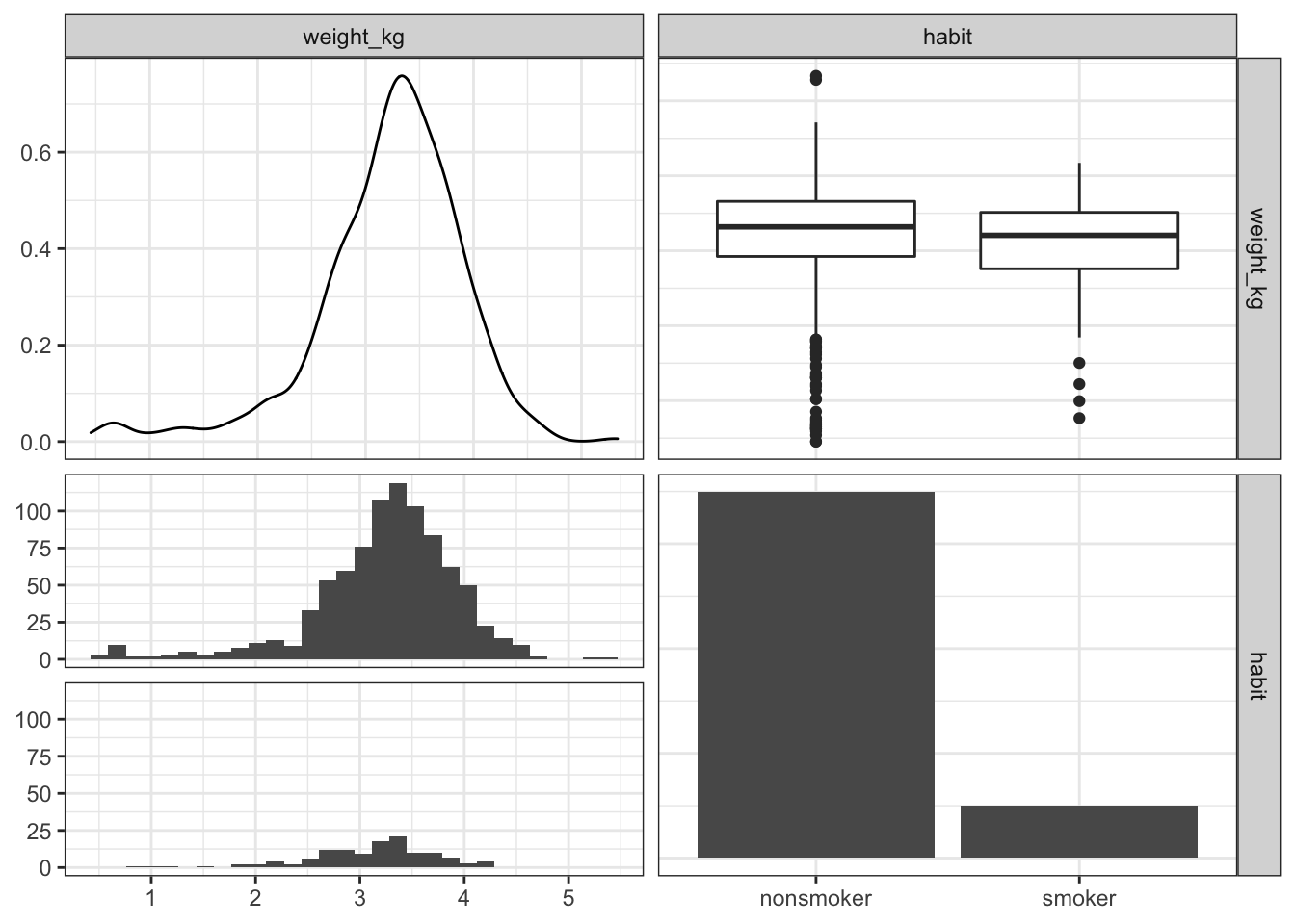
smoking_birth_weight %>%
  filter(!is.na(habit)) %>%
  select(weight_kg, habit ) %>%
  ggpairs()+
  theme_bw()
## `stat_bin()` using `bins = 30`. Pick better value with `binwidth`.
Model building
favstats(~weight_kg, data = smoking_birth_weight)
| min | Q1 | median | Q3 | max | mean | sd | n | missing |
| 0.454 | 2.9 | 3.32 | 3.66 | 5.33 | 3.22 | 0.685 | 1000 | 0 |
model1 <- lm(weight_kg ~ 1, data= smoking_birth_weight)
msummary(model1)
##             Estimate Std. Error t value Pr(>|t|)
## (Intercept)  3.22385    0.02166   148.8   <2e-16 ***
##
## Residual standard error: 0.685 on 999 degrees of freedom
model2 <- lm(weight_kg ~ weeks, data= smoking_birth_weight)
msummary(model2)
##              Estimate Std. Error t value Pr(>|t|)
## (Intercept) -2.767263   0.210948  -13.12   <2e-16 ***
## weeks        0.156325   0.005487   28.49   <2e-16 ***
##
## Residual standard error: 0.5079 on 996 degrees of freedom
##   (2 observations deleted due to missingness)
## Multiple R-squared:  0.449,  Adjusted R-squared:  0.4485
## F-statistic: 811.7 on 1 and 996 DF,  p-value: < 2.2e-16
model3 <- lm(weight_kg ~ weeks + marital, data= smoking_birth_weight)
msummary(model3)
##                     Estimate Std. Error t value Pr(>|t|)
## (Intercept)        -2.795227   0.208616 -13.399  < 2e-16 ***
## weeks               0.154483   0.005437  28.413  < 2e-16 ***
## maritalnot married  0.160758   0.032712   4.914 1.04e-06 ***
##
## Residual standard error: 0.5021 on 995 degrees of freedom
##   (2 observations deleted due to missingness)
## Multiple R-squared:  0.4621, Adjusted R-squared:  0.461
## F-statistic: 427.4 on 2 and 995 DF,  p-value: < 2.2e-16
model4 <- lm(weight_kg ~ weeks + marital + habit, data= smoking_birth_weight)
msummary(model4)
##                     Estimate Std. Error t value Pr(>|t|)
## (Intercept)        -2.784485   0.207877  -13.39  < 2e-16 ***
## weeks               0.154825   0.005418   28.57  < 2e-16 ***
## maritalnot married  0.150470   0.032783    4.59    5e-06 ***
## habitsmoker        -0.139085   0.047961   -2.90  0.00381 **
##
## Residual standard error: 0.5002 on 994 degrees of freedom
##   (2 observations deleted due to missingness)
## Multiple R-squared:  0.4666, Adjusted R-squared:  0.465
## F-statistic: 289.8 on 3 and 994 DF,  p-value: < 2.2e-16
model5 <- lm(weight_kg ~ weeks + marital + habit + whitemom + gender + gained, data= smoking_birth_weight)
msummary(model5)
##                     Estimate Std. Error t value Pr(>|t|)
## (Intercept)        -2.833996   0.207983 -13.626  < 2e-16 ***
## weeks               0.149385   0.005430  27.509  < 2e-16 ***
## maritalnot married  0.120372   0.034381   3.501 0.000485 ***
## habitsmoker        -0.176535   0.047560  -3.712 0.000218 ***
## whitemomwhite       0.096307   0.036921   2.608 0.009236 **
## gendermale          0.171796   0.031313   5.486 5.24e-08 ***
## gained              0.004203   0.001104   3.809 0.000149 ***
##
## Residual standard error: 0.4861 on 963 degrees of freedom
##   (30 observations deleted due to missingness)
## Multiple R-squared:  0.4869, Adjusted R-squared:  0.4837
## F-statistic: 152.3 on 6 and 963 DF,  p-value: < 2.2e-16
model6 <- lm(weight_kg ~ . , data= smoking_birth_weight)
msummary(model6)
##                         Estimate Std. Error t value Pr(>|t|)
## (Intercept)           -1.1422671  0.3381352  -3.378 0.000766 ***
## father_age             0.0038255  0.0035006   1.093 0.274812
## mother_age             0.0001432  0.0045862   0.031 0.975106
## matureyounger mom     -0.0031005  0.0551883  -0.056 0.955212
## weeks                  0.0782526  0.0082420   9.494  < 2e-16 ***
## premiepremie          -0.0200670  0.0653017  -0.307 0.758698
## visits                 0.0004352  0.0040427   0.108 0.914306
## maritalnot married     0.0577704  0.0381095   1.516 0.129945
## gained                 0.0031780  0.0010612   2.995 0.002834 **
## lowbirthweightnot low  1.0853530  0.0648699  16.731  < 2e-16 ***
## gendermale             0.1726791  0.0296218   5.829 8.11e-09 ***
## habitsmoker           -0.0971133  0.0484068  -2.006 0.045177 *
## whitemomwhite          0.1108407  0.0364514   3.041 0.002438 **
##
## Residual standard error: 0.4143 on 787 degrees of freedom
##   (200 observations deleted due to missingness)
## Multiple R-squared:  0.6049, Adjusted R-squared:  0.5989
## F-statistic: 100.4 on 12 and 787 DF,  p-value: < 2.2e-16
huxreg(model1, model2, model3, model4, model5, model6,
       statistics = c('#observations' = 'nobs',
                      'R squared' = 'r.squared',
                      'Adj. R Squared' = 'adj.r.squared',
                      'Residual SE' = 'sigma'),
       bold_signif = 0.05,
       stars = NULL
) %>%
  set_caption('Comparison of models')
Comparison of models
| (1) | (2) | (3) | (4) | (5) | (6) |
| (Intercept) | 3.224 | -2.767 | -2.795 | -2.784 | -2.834 | -1.142 |
| (0.022) | (0.211) | (0.209) | (0.208) | (0.208) | (0.338) |
| weeks | | 0.156 | 0.154 | 0.155 | 0.149 | 0.078 |
| | (0.005) | (0.005) | (0.005) | (0.005) | (0.008) |
| maritalnot married | | | 0.161 | 0.150 | 0.120 | 0.058 |
| | | (0.033) | (0.033) | (0.034) | (0.038) |
| habitsmoker | | | | -0.139 | -0.177 | -0.097 |
| | | | (0.048) | (0.048) | (0.048) |
| whitemomwhite | | | | | 0.096 | 0.111 |
| | | | | (0.037) | (0.036) |
| gendermale | | | | | 0.172 | 0.173 |
| | | | | (0.031) | (0.030) |
| gained | | | | | 0.004 | 0.003 |
| | | | | (0.001) | (0.001) |
| father_age | | | | | | 0.004 |
| | | | | | (0.004) |
| mother_age | | | | | | 0.000 |
| | | | | | (0.005) |
| matureyounger mom | | | | | | -0.003 |
| | | | | | (0.055) |
| premiepremie | | | | | | -0.020 |
| | | | | | (0.065) |
| visits | | | | | | 0.000 |
| | | | | | (0.004) |
| lowbirthweightnot low | | | | | | 1.085 |
| | | | | | (0.065) |
| #observations | 1000 | 998 | 998 | 998 | 970 | 800 |
| R squared | 0.000 | 0.449 | 0.462 | 0.467 | 0.487 | 0.605 |
| Adj. R Squared | 0.000 | 0.448 | 0.461 | 0.465 | 0.484 | 0.599 |
| Residual SE | 0.685 | 0.508 | 0.502 | 0.500 | 0.486 | 0.414 |